curves.m                          

Author: Paul Mennen
Email:  paul@mennen.org
This application (located in the math folder) displays a large variety of planar curves which can be both educational and recreational. Type curves at the command prompt to open the figure window.


Left click on the curve selector popup (The large yellow text in the middle of the lower edge of the figure). That will bring up this menu allowing you to choose one of the 42 curve types. In this example, I have chosen curve #26 which is called the Hypotrochoid, resulting in the figure window shown below.

Rather than picking a particular curve, you may just want to view all the curves in sequence. To do this, instead of left clicking on the curve selector popup, right click it instead. This will advance to the next curve in the sequence. For example, if curve #1 was selected, right clicking on the curve name (popup) will advance to curve #2, without ever opening the popup menu. And the next right click will show you curve #3, etc. Finally, if you are looking at curve #42 (the last one) then right clicking once more will bring you back to curve #1.

Another way to cycle thru all the possible curves is to click the "Cycle" button near the left edge of the figure. It will automatically advance to the next curve every second (by default). This is too fast to read the historical notes for each curve and is more for verifying that the program can correctly display all the curves. You can change the time delay between each curve with the delay popup just below the cycle button. To maximize the "wow" factor, you can set the delay to zero and watch as it cycles thru all 42 curves in about a second.

Note in the figure below that the graph includes six traces, (green, purple, cyan, red, blue, white) corresponding to trace numbers 1 thru 6. The information that curves uses to draw these six traces includes the equation (shown in red immediately below the plot and the 9 parameters shown above the plot (a,b,c,Xoffset,Yoffset,tSteps,tMin,tMax,Style). Actually, it is really 54 parameters, because each of the 9 parameters mentioned are saved independently for each of the six traces. The edit box called "Trace" just to the left of these 9 parameters tells you which of the six sets of 9 parameters you are viewing. It currently shows "1", but as you click on that number it will cycle thru the six traces and you will see that many of these 9 parameters will be changing. As you are doing this you will also notice that the small pointer (<<) to the right of the trace name moves to the trace whose parameters are being displayed.

All 54 parameters for each of the 42 curve types as well as the equation itself and the historical notes that appear when the curve type is selected are all stored in the curves.m source code which explains why curves.m is one of the longer programs in the toolbox (330 lines of code/data).

The ability to modify these 54 parameters for various curve types while observing the effects of these changes accounts for this program's educational value - and sometimes recreational value as well. For example, if you select curve #36, this program essentially becomes a Spirograph toy. Changing the a, b, and c parameters is like choosing the sizes of the two gears and the length of the pen arm. You can create all figures possible with a Spirograph as well as some that the Spirograph can't produce.

All 2268 parameters (54 x 42 curves) are individually stored in the program and will be preserved until you right click on the defaults button. That resets all 2268 parameters to the default values. (Actually, there really are fewer than 2268 parameters since many of the curve types don't use all six traces.) Left clicking on the default button resets only the currently viewed curve type to the default values. When you exit the program any changes you have made to all these parameters are lost and so are reset to the default values when the program is restarted.

Note that the equations defining the curves always contain the variable t, because that is the independent variable. It is computed based on the tMin, tMax, & tSteps parameters with the Matlab expression t = tMin : (tMax-tMin)/tSteps : tMax.

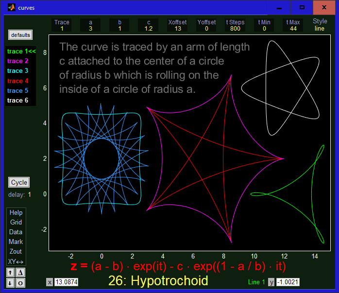
In this example, the equation defines the variable z, where z is always taken to be a complex quantity. The real part of z will of course be plotted along the x axis and the imaginary part of z will be plotted along the y axis.

The equations for many of the other curves will define the variable r which means the curve has been defined using polar coordinates (i.e. r is the radius or distance from the origin, and t is theta, i.e. the angle from the x axis measured in radians). Instead of defining z or r, some of the equations will explicitly define both x and y in terms of t.

The equations shown in red below the plot appear as standard Matlab expressions of the vector t and the parameters a, b, and c except for three syntax changes to improve readability: Although not shown in the equations, the parameter Xoffset is added to the x coordinate and the parameter Yoffset is added to the y coordinate. These offsets allow us to position the six traces in different (usually non-overlapping) regions of the plot.

This application is a good example of how a graphical interface can benefit from the pseudo edit object. If we used traditional Matlab graphical objects for the ten controls and labels at the top edge of the figure these controls would take up much more space resulting in a smaller plotting area. Also, the increment/decrement feature of the pseudo edit object proves valuable here. I recommend checking out the The pseudo edit object section to improve your understanding of how to use this pseudo object.

If you have any questions about the use or coding of this application, don't hesitate to contact me at the email address shown at the top of the page.

Copyright © 2023
Paul Mennen